12 Manifolds, homeomorphism, and neural networks
This chapter covers
- Introduction to manifolds
- Introduction to homeomorphism
- Role of manifolds and homeomorphism in neural networks
This is a short chapter that briefly introduces (barely scratching the surface of) a topic that could fill an entire mathematics textbook. A rigorous or even comprehensive treatment of manifolds is beyond the scope of this book. Instead, this chapter primarily focuses on geometric intuitions required for deep learning.
12.1 Manifolds
A manifold is a generalization of the notions of curve, surface, and volume into a unified concept that works in arbitrary dimensions. In machine learning, the input space can be viewed as a manifold. Usually, the input manifold is not very conducive to classification. We need to transform (map) that manifold to a different manifold that is friendlier to the classification problem at hand. This is what a neural network does.
In a multilayered neural network, each layer transforms (maps) from one manifold to another. For the classification problem, the end manifold is expected to be one where the classes can be separated by a linear surface (hyperplane). The last layer provides this linear separator. Figure 12.1 provides an example of a transformation to a space where classification is easier.
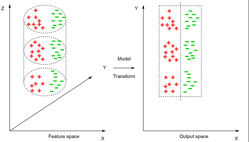
Figure 12.1 The input points lie on a cylindrical manifold (surface). Here, the two input classes (indicated by + and -, respectively) cannot be separated linearly. If we unroll (map) the cylinder surface into a plane, the two classes can be separated linearly.
Unlike physical surfaces we see and touch in everyday life, manifolds are not limited to three dimensions. Human imagination may fail in visualizing higher-dimension manifolds, but we can typically use three-dimensional analogies as surrogates—they often work, although not always. A neural network layer or sequence of layers can be viewed as mapping points from one manifold to another.
Manifolds are locally Euclidean. To get an intuitive understanding of this, imagine a circle with a very thin string wrapped around it. Now, take any point on the circle and take a small arc of the circle containing that point. If we cut off the portion of the string corresponding to that segment, we can straighten that little piece of string into a straight line without twisting or tearing it. In other words, the small neighborhood on the circle around the chosen point has 1:1 mapping with a line segment. All points on the circle satisfy this property. Such a curve is said to be locally Euclidean. The concept can be extended to higher dimensions. Consider the surface of a sphere (this is an example of a 2-manifold). Imagine a rubber sheet tightly fitted around the sphere. Take an arbitrary point and a small patch of the spherical surface containing the point (see figure 12.2c). If we cut off the rubber sheet corresponding to the patch, it can be flattened into a plane without twisting or tearing. So, the sphere surface is locally Euclidean. The torus surface (donut-shaped object) is another example of a 2-manifold. In general, d-manifold is a space (set of points) on which every point has a small neighborhood of points in the space that contains the point and can be mapped 1:1 to ℝd without twisting or tearing. For instance, a circle is a 1D manifold, and every point on it has a container arc that can be mapped to a line (ℝ1). A sphere surface is 2D manifold, and every point of it has a containing patch that maps 1:1 to a plane (ℝ2). We say manifolds are locally Euclidean. Figure 12.2 illustrates the concept.
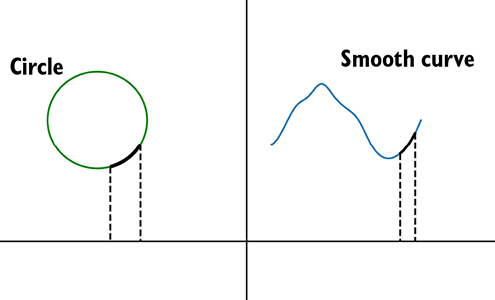
(a) Any arbitrary continuous curve (for example, a circle) is a 1D manifold.
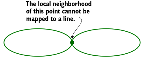
(b) The 8-curve is a non-manifold. The χ-shaped neighborhood of the marked point cannot be mapped 1 : 1 to a straight-line segment.
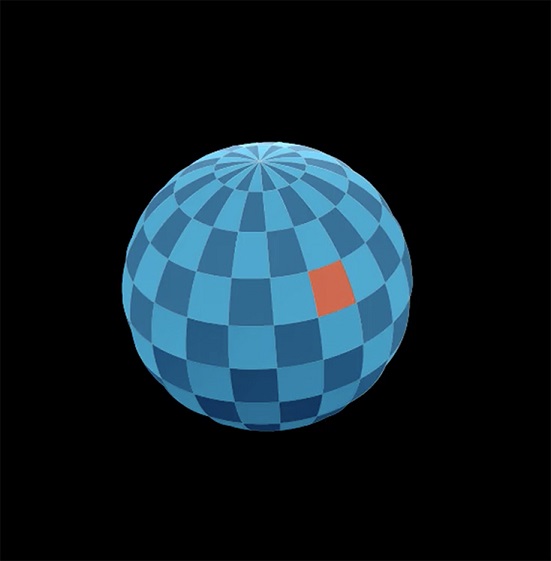
(c) A sphere is an example of a 2-manifold.
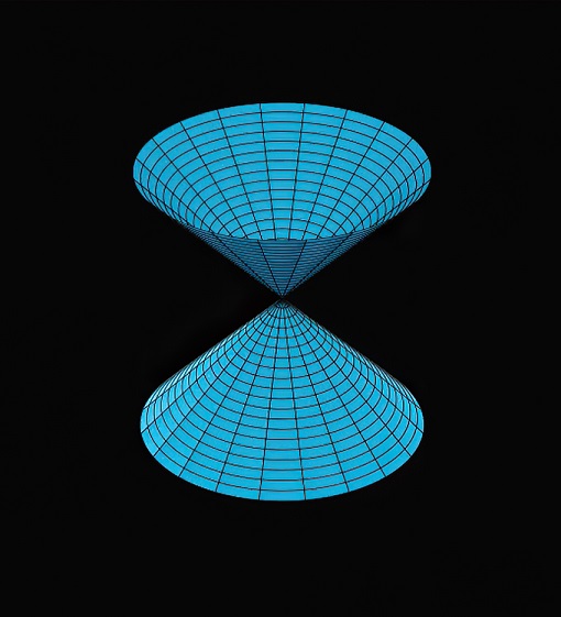
(d) An hourglass is an example of 2D non- manifold surface.
Figure 12.2 Manifolds and non-manifolds in 1D and 2D
A little thought will reveal that the locally Euclidean property makes calculus possible. For instance, how do we compute the area under a curve, f(x) in the interval x = a and x = b? The formula is ∫x=ax=b f(x) dx. We take infinitesimally small segments of the curve and pretend they are straight lines, which can be projected onto a tiny line segment on the X axis. The resulting narrow quadrilateral can be approximated by a rectangle whose sides are parallel to the X and Y axes. We sum (integrate) the areas of all the tiny rectangles that cover the same area as the one we are computing (see figure 12.3). This scheme depends on the ability to represent tiny segments of the curve as straight lines. A similar case can be made about computing the length of the curve segment. In higher dimensions, the same idea applies: calculus is dependent on the ability to pretend that a curve or surface can be locally approximated by something flat. The graph of any continuous vector function ![]() = f(
= f(![]() ), where
), where ![]() is any open subset of ℝn—that is,
is any open subset of ℝn—that is, ![]() ∈ 𝕌 ⊂ ℝn and f(
∈ 𝕌 ⊂ ℝn and f(![]() ) ∈ ℝm—yields a manifold in (
) ∈ ℝm—yields a manifold in (![]() ,
, ![]() ) in ℝm × ℝn.
) in ℝm × ℝn.
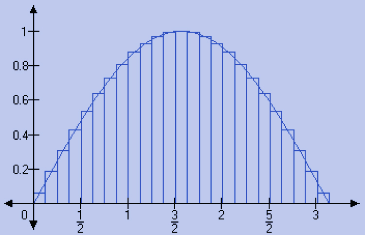
Figure 12.3 Area under a curve is computed by locally approximating curve segment with tiny straight lines—needs locally Euclidean property
In this context, note that the entire sphere cannot be mapped to a plane (try opening the sphere onto a plane). This is why it is impossible to draw a perfect map of the globe on a piece of paper with all regions drawn to scale. Typically, the polar regions occupy areas disproportionately large on the paper map. But small patches on the spherical surface can be mapped onto planes, which is enough to call this surface a manifold. Hence the word local in locally Euclidean.
12.1.1 Hausdorff property
Manifolds usually have another property, known as the Hausdorff property. If we take any pair of points on a manifold—no matter how close they are—we can find a pair of disjoint neighborhoods around the respective points consisting entirely of points on the manifold. Loosely speaking, this means if we take any pair of points on the manifold, we can find an infinite number of points between them, all belonging to the manifold. This is illustrated in figure 12.4. It’s easy to see that this is true for the real line (ℝ1): take any pair of points, and there are enough points between them to create a disjoint pair of neighborhoods centered on each.
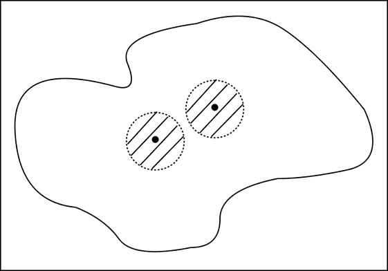
Figure 12.4 for any pair of points, we can find a disjoint neighborhood pair containing the respective points and consisting of points from the manifold.
12.1.2 Second countable property
Manifolds are second-countable. To explain this, we will first briefly outline a few concepts. (Disclaimer: the following explanations err toward ease of understanding as opposed to mathematical rigor.)
Open sets, closed sets, and boundaries
Consider the set of points belonging to the interval A ≡ 0 < x < 1 (you can imagine it to be a segment of the real line). Take any point in this set A, say x = 0.93. You can find a point on its left (say, 0.92) and on its right say, 0.94), both of which are in the same set A. In some sense, the point is surrounded by points belonging to the same set. Hence it is an internal point. The funny thing is, in this set, all points are internal. In comparison, consider the set Ac ≡ 0 ≤ x ≤ 1. This includes the previous set A as well as the boundary points x = 0 and x = 1. Note that the boundary points can be approached from both inside and outside the set A. If we take a small neighborhood of any point in the boundary, consisting of all points within a small distance ϵ, there are points inside and outside A. A is an open set. If we add its boundary to itself, it becomes a closed set Ac.
The concept extends to higher dimensions. For instance, the set of 2D points belonging to the unit disc S ≡ x2 + y2 < 1 is an open set. If we add the boundary—the circle Sc ≡ x2 + y2 = 1—we get a closed set. All this is illustrated in figure 12.5.
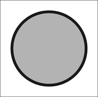
Figure 12.5 The open set, disk without a boundary is shown in gray. The boundary is shown in black. Gray+black is the closed set.
Bounded, compact, and precompact sets
A set is said to be bounded if all its points lie within a fixed distance of each other. The sets A, Ac, and S, Sc discussed previously are bounded. A compact set is bounded as well as closed. The sets Ac and Sc are compact. And a set is precompact if it can be converted into a compact set by just adding its boundary (for example, A and S). Note that not all open sets are precompact: for example, −∞ < x < ∞ is open but not precompact. All precompact sets are open, however.
Manifolds may or may not include a boundary. A disc is a 2-manifold with a boundary. Its boundary is the circle’s circumference, which is a 1-manifold. A three-dimensional ball is a 3-manifold with a boundary. The boundary is the surface of the sphere, which is a 2-manifold. The open set of points on the disc sans the boundary is also a 2-manifold. A square area is a 2-manifold with a boundary whose boundary is the square, which is a 1-manifold. A three-dimensional cube is a 3-manifold with a boundary whose boundary is a 2-manifold corresponding to the surface of the cube. In general, the boundary of a d-manifold with boundary is a d − 1-manifold.
Now, let’s go back to the second countable property of manifolds. The second countable property of a manifold implies that every manifold has a basis of open sets. This means for every manifold M, there exists a countable collection U ≡ {Ui}, where Ui are precompact subsets of M and any open subsets of M can be expressed as a union of elements of U. This is illustrated in figure 12.6.
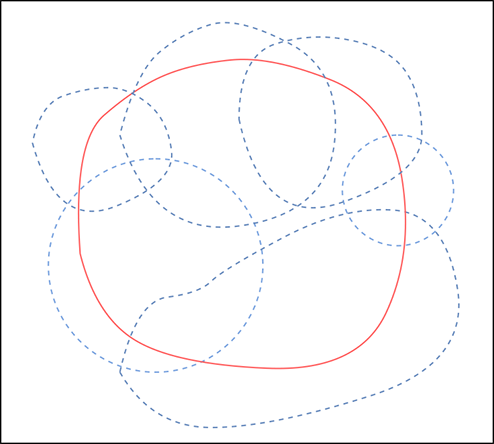
Figure 12.6 ball-bounded areas.
12.2 Homeomorphism
We have been speaking about 1:1 mappings between an arc of a circle and a line segment. If we have a piece of string tightly fitted on the arc, all we have to do is to grab the string’s two ends and pull it out to get the corresponding straight line—we do not have to do any twisting or tearing (see the black arc in figure 12.2). Similarly, the mapping between a patch on the surface of a sphere can be mapped 1:1 to a plane by simply pulling an imaginary rubber sheet fitted on the patch (see the patch in figure 12.2c). These are examples of a general class of mappings called homeomorphism. Formally, a homeomorphic mapping comprises a pair of functions f and f−1 between two sets of points X and Y such that
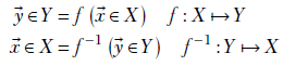
where
-
f is 1:1: it maps each
 to a unique
  , and distinct s are mapped to distinct s.
 -
f−1 is 1:1: it maps each
to an unique , and distinct s are mapped to distinct s. -
f is a continuous function: it maps nearby values of
to nearby values of . -
f−1 is continuous function: it maps nearby values of
to nearby values of .
An intuitive way to visualize homeomorphism is that it transforms one manifold to another by stretching or squishing but never by cutting, breaking, or folding. Homeomorphism preserves path-connectedness. A set of points is said to be path-connected if a path between any pair of them exists, comprising points belonging to the set.
12.3 Neural networks and homeomorphism between manifolds
Consider two classes A and B defined on the real line:
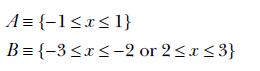
The 1-manifolds corresponding to these classes are not clearly separable in their original space (see figure 12.7a) because class A is “surrounded” by class B. But if we pinch the origin and pull it up—in other words, perform a specific homeomorphism—to transform it, as shown in figure 12.7c, it is possible to separate the transformed manifolds with a straight line. Similarly, figure 12.7b shows two classes A and B:
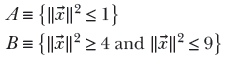
These are 2-manifolds that are hard to separate in their original space because, again, class B surrounds class A. But if we pinch and pull the origin to create the manifolds shown in figure 12.7d, they become separable by a plane (see figure 12.7d).
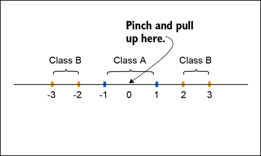
(a) A linear classifier cannot separate points on the line.
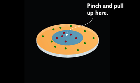
(b) A linear classifier cannot separate points on the disk.
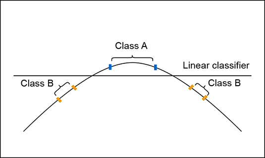
(c) Lines transformed to a curved shape allow classification with a linear classifier (line).
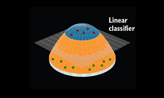
(d) Disks transformed to a 3D bell-like shape allow classification with a linear classifier (plane).
Figure 12.7 Homeomorphism to a friendlier manifold can help the classification.
A linear layer of a neural network does the following transformation discussed in detail in equation 8.7):
![]()
Note that all of these operations, multiplication with the weight matrix W, translation by ![]() , and the sigmoid nonlinearity are continuous invertible functions. Hence, they are homeomorphisms. The composite operation where these are applied in sequence is another homeomorphism. (Strictly speaking, multiplication by a weight matrix is invertible only when the weight matrix W is square with a nonzero determinant. And if the weight matrix has a zero determinant, the layer effectively does a dimensionality reduction.)
, and the sigmoid nonlinearity are continuous invertible functions. Hence, they are homeomorphisms. The composite operation where these are applied in sequence is another homeomorphism. (Strictly speaking, multiplication by a weight matrix is invertible only when the weight matrix W is square with a nonzero determinant. And if the weight matrix has a zero determinant, the layer effectively does a dimensionality reduction.)
One way to view a multilayered neural network is that the successive layers homeomorphically transform the input manifold so that it becomes easier and easier to separate the classes. The final layer may be a simple linear separator (as in figure 12.7).
Summary
-
A manifold is a hyperdimensional collection of points space) that satisfies three properties: locally Euclidean, Hausdorff, and second countable.
-
A d-manifold is a space in which every point has a small neighborhood that contains the point and can be mapped 1:1 to a subregion of ℝd without folding, twisting, or tearing. In other words, the local neighborhood around any point on a manifold can be approximated by something flat. For instance, a continuous curve in 3D space is a 1-manifold: if we imagine the curve as a string, any local neighborhood is a substring that can be pulled and straightened into a straight line. Any continuous surface in 3D is a 2-manifold: if we imagine the surface as a rubber membrane, any local neighborhood can be pulled and stretched into a flat planar patch. This property (the ability to pretend that a curve or a surface can be locally replaced by a linear piece) is what enables us to perform calculus.
-
Homeomorphism is a special class of transformation mapping) that transforms one manifold to another via stretching/squishing without tearing, breaking, or folding.
-
Homeomorphism preserves path-connectedness.
-
Roughly speaking, a neural network layer can be viewed as a homeomorphic transform that maps points from its input manifold to an output manifold that is (hopefully) more suitable for the end goal. The entire multilayered perceptron (neural network) can be viewed as a sequence of homeomorphisms that, in a series of steps, transform the input manifold to a manifold that makes the end goal easier. In particular, a classifier neural network maps the input manifold to an output manifold where the points belonging to different classes are well-separated.